The Fundamental Theorem of Algebra via Connectedness

It is intuitive that removing even a single point from a line disconnects it, but removing a finite set of points from a plane leaves it connected.

However, this basic fact leads to a non-trivial property of real and complex polynomials: not all non-constant real polynomials have real roots, but all non-constant complex polynomials have complex roots. The latter, is in fact the fundamental theorem of algebra:

We’ll prove this theorem using nothing stronger than the complex inverse function theorem. Here’s a synopsis:

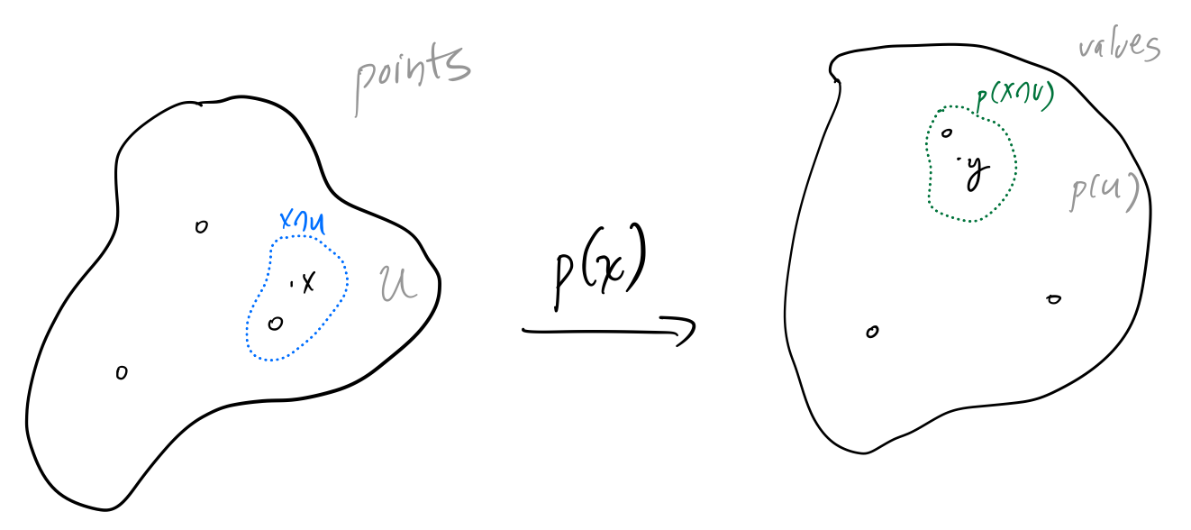
1. Let p \colon \mathbb{C}→ \mathbb{C} be a non-constant complex polynomial, and V_{\text{regular}} its set of regular values. Let P_{\text{pure}}= p^{-1}(V_{\text{regular}}) be its set of pure regular points, so that p can be thought of a P_{\text{pure}}→ V_{\text{regular}} map.
2. Any complex polynomial, and p in particular, is a closed \mathbb{C}→ \mathbb{C} map, and thus also a closed P_{\text{pure}}→ V_{\text{regular}} map.
3. Furthermore, by the inverse function theorem, p is an open P_{\text{regular}}→ V_{\text{regular}} map, and thus also an open P_{\text{pure}}→ V_{\text{regular}} map.
4. p, being non-constant, has only finitely many critical points. (This is the step that fails for real polynomials.) Therefore, V_{\text{regular}} is the complex plane with a finite set of points removed, and thus is connected. Similarly, P_{\text{pure}} is also connected.
5. p, being a continuous, open, and closed P_{\text{pure}}→ V_{\text{regular}} map, must take connected components to connected components. Since P_{\text{pure}} and V_{\text{regular}} are both connected, that means that p maps P_{\text{pure}} onto V_{\text{regular}}.
6. p also maps P_{\text{critical}} onto V_{\text{critical}}, so p is surjective on \mathbb{C}, and thus must have a root.

This is a wonderfully succinct proof, but it’s full of subtleties and would benefit from elaboration (as well as some diagrams). We’ll do that in the rest of this article. First, we need some definitions.

Points and values

If a function f(x) maps from A to B, we’ll call elements of A points and elements of B values; in our case, A and B will both be subsets of either \mathbb{R} or \mathbb{C}, but it’s helpful to distinguish when we’re talking about a real or complex number as a domain element versus a codomain element.

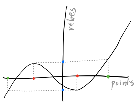
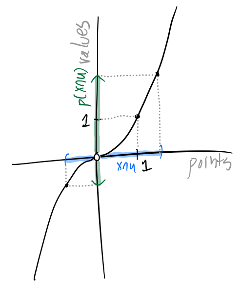
If f(x) is differentiable, we’ll call x a critical point if f'(x) = 0 and a regular point otherwise. We’ll call y a critical value if y = f(x) for some critical point x and a regular value otherwise. In particular, if y is not in the image of f, then y is a regular value.

A regular point may map to a critical value. In that case, we call it an impure regular point and a pure regular point otherwise. (This is nonstandard terminology, but it helps with visualizing what’s going on.)

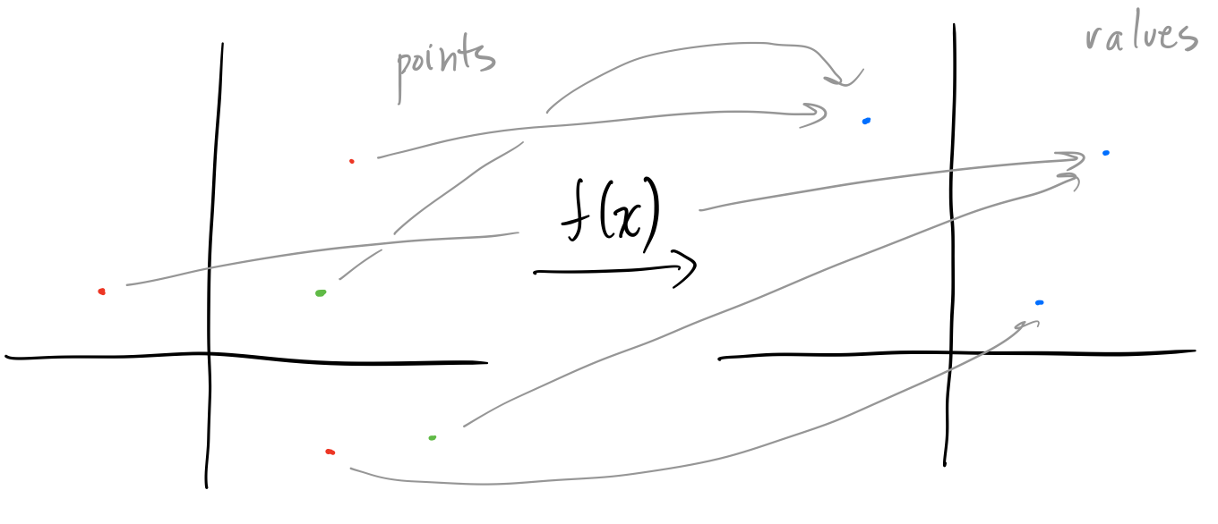
The strategy of the proof is to show that a non-constant complex polynomial f(x) is surjective. By construction, f(x) maps impure regular points and critical points onto the critical values. Then it suffices to show that f(x) maps the pure regular points P_{\text{pure}} onto the regular values V_{\text{regular}}. In doing so, we’ll show that there are only a finite number of critical points, critical values, and impure regular points; therefore, P_{\text{pure}} is the complex plane minus a finite number of points, and that is where connectedness comes into play.

Connected sets

A subset X of a topological space is disconnected if it is the union of two disjoint, non-empty open sets, and connected otherwise.

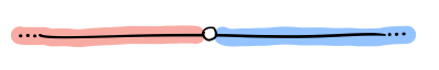
For example, the set X in the first figure is the real line \mathbb{R} with a single point a removed. Then X = (-∞, a) ∪ (a, ∞), so it is disconnected.

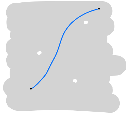
It is harder to show that a set is connected. However, we can use a stronger property that’s easier to show. A subset X of a topological space is path-connected if for every two points x and y in X, there exists a path from x to y—that is, a continuous function f \colon [0, 1] → X such that f(0) = x and f(1) = y. A path-connected set is automatically a connected set—being able to draw paths between any two points makes it impossible to split the set into two disjoint non-empty open subsets.

In particular, let X be the plane \mathbb{R}^2 or \mathbb{C} with a finite number of points p_i removed. Then we’ll show that X is path-connected. Let d be the minimum distance between any of the removed points, and let r = d/3. Then given x and y in X, let f be the straight-line path from x to y. For any p_i that is on f, replace the segment through p_i with a semi-circular arc of radius r around p_i. Since r < d/2, the arc will not have any other removed point on it, and no two arcs will overlap. Therefore, this modified path lies entirely in X. Since x and y were arbitrary, X is path-connected, and thus connected.

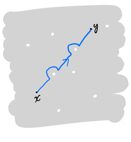
We’re most interested in connected sets that are maximal in the sense that they’re not contained in a larger connected set. These are called connected components, and any topological space can be decomposed into its connected components. For example, the set X in the first figure has two connected components (-∞, a), (a, ∞), and the plane with a finite number of points removed remains connected, and thus only has a single connected component. However, removing a line from a plane splits it into two connected components, one on each side of the line.

A continuous function preserves connectedness: it maps connected sets to connected sets. However, it may map a connected component to a connected set that’s not a connected component. We want to show that real and complex polynomials map connected components to connected components—this leads us to the concepts of open and closed maps.

Open and closed functions

If a function f(x) between topological spaces A and B sends open sets of A to open sets of B, we call it open. Similarly, if it sends closed sets of A to closed sets of B, we call it closed. Be careful! Like with sets, whether a function is open is unrelated to whether it is closed; a function may be neither open nor closed, just open, just closed, or both.

We’re more interested in sets and functions that are both open and closed, which we’ll call clopen. A topological space A always has two clopen subsets: \emptyset and itself. However, if its disconnected, it may have more: in general, a clopen subset X is a union of connected components of A. Conversely, if A has finitely many connected components, each connected component is clopen.

Then since a clopen function f(x) between A and B sends clopen sets of A to clopen sets of B, it then sends connected components of A to unions of connected components of B. If f(x) is also continuous, then it must send a connected component of A to another connected set, which then must be a connected component of B.

Therefore, since real and complex polynomials are continuous, in order to show that they map connected components to connected components, we need to show that they are also clopen.

Real and complex polynomials are closed

First, we want to show that a real polynomial p(x) \colon \mathbb{R}→ \mathbb{R} or a complex polynomial p(x) \colon \mathbb{C}→ \mathbb{C} is closed.

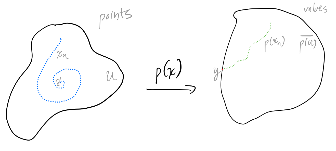
If p(x) is constant, then this follows immediately. Otherwise, the essential property of polynomials that we use is that if x → ∞, then p(x) → ∞. In other words, if x_n is a sequence such that p(x_n) is bounded, then x_n must also be bounded.

Then let U be a closed set of points, and let y ∈ \overline{p(U)}; in other words, y is a limit point of p(U). To show that p(U) is closed, we want to show that y is in fact in p(U). Since y is a limit point of p(U), there is some sequence x_n in U such that p(x_n) converges to y. Then p(x_n) is bounded, so by the above, x_n is also bounded. Then some subsequence x_m of x_n converges to some \tilde{x} ∈ U. Since p is continuous, p(x_m) then converges to p(\tilde{x}), which must then equal y. Therefore, y is indeed in p(U), which shows that p(x) is a closed map.

So polynomials \mathbb{R}→ \mathbb{R} or \mathbb{C}→ \mathbb{C} are closed, but what we really want to show is that they’re also closed as maps from its pure regular points P_{\text{pure}} to its regular values V_{\text{regular}}. In general, restricting the domain or codomain of a function doesn’t preserve the property of being closed, but if f is a closed map from A to B and D ⊆ B, then f is a closed map from C = f^{-1}(D) to D.

A proof: if U is a closed subset of C, then it is U' ∩ C for U' a closed subset of A. In general we have the identity f(X ∩ Y) ⊆ f(X) ∩ f(Y), so f(U' ∩ C) ⊆ f(U') ∩ f(C) ⊆ f(U') ∩ D\text{.}

Conversely, if y ∈ f(U') ∩ D, then f(x) = y for some x ∈ U'. Since f(x) ∈ D, x ∈ C = f^{-1}(D), so x ∈ U' ∩ C. Therefore, y ∈ f(U' ∩ C), thus f(U') ∩ D ⊆ f(U' ∩ C), and

f(U) = f(U' ∩ C) = f(U') ∩ D\text{.}

f(U') is a closed subset of B by f being closed, and so f(U') ∩ D is a closed subset of D.

In particular, P_{\text{pure}} is the inverse image of V_{\text{regular}} by construction, so a real or complex polynomial is thus a closed map from P_{\text{pure}} to V_{\text{regular}}.

Real and complex polynomials have finitely many critical points

One subtle but important fact that we need is that non-constant real and complex polynomials have finitely many critical points. A critical point of the real or complex polynomial p(x) is a root of p'(x), which is another polynomial, so the statement that a non-constant real or complex polynomial has finitely many critical points is equivalent to the statement that a non-zero real or complex polynomial has finitely many roots.

But isn’t that equivalent to the fundamental theorem of algebra? No! For one, it’s also true for real polynomials. More generally, it’s an upper bound on the number of roots, whereas the fundamental theorem of algebra is a lower bound.

If a real or complex polynomial p(x) of positive degree n has a root r, then p(x) = (x - r) q(x) for some polynomial q(x) of degree n - 1. Then since non-zero degree-0 polynomials have no roots, by induction p(x) has at most n roots.

Therefore, a non-constant real or complex polynomial of degree n has at most n - 1 critical points.

Real and complex polynomials are open on regular points

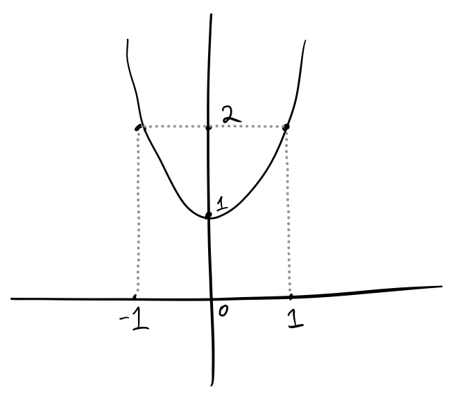
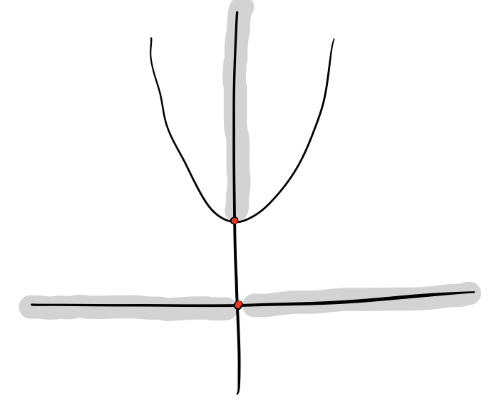
A real polynomial p(x) \colon \mathbb{R}→ \mathbb{R} is not open in general; a figure above shows that p(x) = x^2 + 1 is a counterexample. Fortunately, it’s only the critical points that are the problem: as functions from P_{\text{regular}} to \mathbb{R}, real polynomials are open.

The complex case is actually easier—the open mapping theorem implies that a complex polynomial p(x) \colon \mathbb{C}→ \mathbb{C} is open in general. However, that theorem uses a bit more complex analysis machinery than we’d like—it turns out that we can use the same proof as in the real case (which is simpler) to show that complex polynomials are open as functions from P_{\text{regular}} to \mathbb{C}.

So let’s start the proof. Let p(x) be a real (or complex) polynomial, considered as a function from V_{\text{regular}} to \mathbb{R} (or \mathbb{C}). Let U ⊆ V_{\text{regular}} be open, and we want to show that p(U) is also open.

Let y ∈ p(U). Then y = p(x) for some regular point x ∈ U. Since p'(x) ≠ 0, by the real inverse function theorem (or the complex inverse function theorem) there is some open set X containing x that is diffeomorphic to p(X).

U is open in V_{\text{regular}}, which is \mathbb{C} minus a finite number of points. Therefore, U is an open set in \mathbb{C} minus a finite number of points, and is thus also open in \mathbb{C}. (This is where we use the fact that p(x) has a finite number of critical points.)

Since U is open in \mathbb{C}, so is X ∩ U, which is diffeomorphic to p(X ∩ U), which is thus an open set contained in p(U) containing y. Since y was arbitrary, p(U) is open.

Since a real or complex polynomial p(x) is open from P_{\text{regular}} to \mathbb{R} or \mathbb{C}, the same reasoning as in the closed case shows that since V_{\text{regular}}⊆ \mathbb{C} and P_{\text{pure}}= p^{-1}(V_{\text{regular}}), then a real or complex polynomial is an open map from P_{\text{pure}} to V_{\text{regular}}.

Non-constant complex polynomials are surjective (but not real ones)

Now we’re ready to put it all together. Let p(x) be a non-constant complex polynomial. By the above, it is clopen as a map from P_{\text{pure}} to V_{\text{regular}}. Therefore, since it’s also continuous, it maps each connected components of P_{\text{pure}} to a connected component of V_{\text{regular}}. But both P_{\text{pure}} and V_{\text{regular}} are \mathbb{C} minus a finite set of points, and thus they both have a single connected component. Therefore, p(x) maps P_{\text{pure}} onto V_{\text{regular}}. Since it also maps P_{\text{critical}} onto V_{\text{critical}}, it maps \mathbb{C} onto \mathbb{C}= V_{\text{critical}}∪ V_{\text{regular}}.

In particular, this implies that p(x) has a root, which is the fundamental theorem of algebra.

What about the real case? Consider the real polynomial p(x) = x^2 + 1. It has a single critical value 1 mapped to by a single critical point 0, so P_{\text{pure}} has two connected components: (-∞, 0) and (0, ∞). V_{\text{regular}} has two connected components (-∞, 1) and (1, ∞), but p(x) maps both connected components of P_{\text{pure}} to (1, ∞), and so isn’t surjective on \mathbb{R}, and in particular doesn’t have a root.

Further reading

This MathOverflow answer is where I first found this proof, although it’s slightly less elementary (it relies on polynomials being proper) and even more terse.

Milnor’s wonderful book “Topology from the Differentiable Viewpoint” has a similarly elegant proof using the fact that a sphere minus a finite number of points remains connected, whereas a circle minus at least two points becomes disconnected. However, it requires somewhat more machinery.

This set of notes is a self-contained proof of the inverse function theorem for \mathbb{R}^n (note that the inverse function theorem for \mathbb{C} reduces to the inverse function theorem for \mathbb{R}^2 by the Cauchy-Riemann equations.) It turns out that a property called “local surjectivity” is all that’s needed to prove openness, but that’s less well-known and only slightly less complicated than the full inverse function theorem.