Sampling the Visible Sphere

(Note: this article is a summary of this thread on ompf2.)

The usual method for sampling a sphere from a point outside the sphere is to calculate the angle of the cone of the visible portion and uniformly sample within that cone, as described in Shirley/Wang.

However, one detail that is glossed over is that you still need to map from the sampled direction to the point on the sphere. The usual method is to simply generate a ray from the point and the sampled direction and intersect it with the sphere. However, this intersection test may fail due to floating point inaccuracies (e.g., if the sphere is small and the distance from the point is large).

I've found a couple of existing ways to deal with this. As described in the pbrt book, pbrt simply assumes that the ray just grazes the sphere if the intersection fails, and then projects the center of the sphere onto the ray (code here). mitsuba moves the origin of the ray closer to the sphere (in fact, from within it) before doing the test (falling back to projecting the center onto the ray if that still fails) (code here).

However, this seems inelegant. I've come up with a better way, which involves converting the sampled cone angle \(θ\) (as measured from the segment connecting the point to the sphere center) into an angle \(α\) from the inside of the sphere, and then simply using \(α\) and the sampled polar angle \(\varphi\) onto the sphere. This turns out to be simple, and in my unscientific tests a bit faster.

Here's a crude diagram showing the geometry:

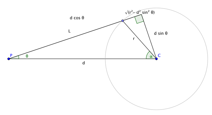
You can see that \[ L = d \cos θ - \sqrt{r^2 - d^2 \sin^2 θ} \] and also by the law of cosines, \[ L^2 = d^2 + r^2 - 2 d r \cos α\text{.} \] We're actually more interested in \(\cos α\), so solving for that we get \[ \cos α = \frac{d}{r} \sin^2 θ + \cos θ \sqrt{1 - \frac{d^2}{r^2} \sin^2 θ}\text{.} \] An alternate form, which may be easier to analyze, recalling that \(\sin θ_{\max} = r/d\), is \[ \cos α = \frac{\sin^2 θ}{\sin θ_{\max}} + \cos θ \sqrt{1 - \frac{\sin^2 θ}{\sin^2 θ_{\max}}}\text{.} \]

(cos θ, φ) = uniformSampleCone(rng, cos θmax)
D = 1 - d² sin² θ / r²
if D ≤ 0 {
  cos α = sin θmax
} else {
  cos α = (d/r) sin² θ + cos θ √D
}
ω = sphericalDirection(cos α, φ)
pSurface = C + r ω

There's no backfacing since we clamp \(\cos α\) to \(\sin θ_{\max}\), which is analogous to the case when the ray from \(P\) misses the sphere.

Note that one cannot just compute \(α_{\max}\) and uniformly sample the cone from inside the sphere, as that doesn't produce the same distribution over the visible region as sampling the cone from outside the sphere. To preserve correctness, you would have to use the (uniform) PDF over the surface area of the visible portion of the sphere, but you would have to then convert that to a PDF with respect to projected solid angle from \(P\), which is suboptimal to just doing the sampling with respect to projected solid angle from \(P\) as described above.

Like this post? Subscribe to my feed or follow me on Twitter .